Gas Material Balances and Straight Line Methods
1) Gas-in-place with water influx
In prior discussion of MBE, we multipled Gp by Bg, the formation
volume factor to obtain a reservoir volume in either cubic ft or bbls. Remember
the constant 0.02829 was used to calculate Bg in cubic ft, and 0.00504 for barrels.
 Recovery
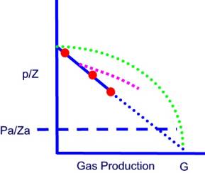
of a dry gas with adequate production history and no water influx, can be determined
by the P/Z verses Gp plot. Overestimation of OGIP and ultimate recovery is
possible in the case of a geopressured formation (green line) or water influx
(purple line).
Recovery
of a dry gas with adequate production history and no water influx, can be determined
by the P/Z verses Gp plot. Overestimation of OGIP and ultimate recovery is
possible in the case of a geopressured formation (green line) or water influx
(purple line).
The pressure support from an aquifer may not be apparent at first. Assuming
no water influx when one is present can result in over estimation of both gas
in place and ultimate recovery.
In the plot above, Pa is the abandonment pressure, with corresponding Za factor.
Frequently, the abandonment point is based more on economics, which may relate
to the gas production from several fields.
From straight line MB methods, we intend to calculate GIIP and cumulative
water influx, We. This is a function of aquifer’s geometry and transmissibility
T = Kh. Aquifers may initially provide complete support or partial support
depending on these characteristics.

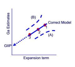 The
next graph has purposely been left unlabeled.
The
next graph has purposely been left unlabeled.
This of course, is the straight line approach to material balance, and the
correct model has the right cumulative water influx, We. The points are labeled
1, 2 and 3, to show the time sequence. You can think of water influx as the
opposite of production.
With Line (B), it appears that we will over estimate gas in place. Therefore,
we must be using an We that is too high or too low? Think for a moment before
proceeding.
Congratulations! We is too low. Just as the gas-in-place is too high when we
neglect completely neglect water influx in the P/Z method, GIIP is overestimated
when we underestimate it.
The straight line equation for gas reservoir with water influx is:
See Reference 1, equation 10.77, on page 244.
The f(p ,t) term is the aquifer model, which can be either steady-state
or unsteady state.
Steady-state model for aquifer
The steady-state model means that the aquifer keeps up with production. Perhaps
initially, the field declines in pressure and rates drop off. At this point,
the total voidage in the reservoir equals the influx from the aquifer and the
pressure stabilizes. In the steady state model, water influx rate (that is the
derivative of We with time), is in proportion to the pressure drop. Under this
condition, the water influx rate must equal the gas and water rate, all expressed
in reservoir units.
Example seen in Reference 4, page 277. The example given is for an oil field,
so the released free gas and oil production must be accounted included in the
We calculation. Note the conclusion of the authors of reference 4, page 280:
“In nearly all applications, the steady state models discussed in the previous
section are not adequate in describing the water influx.”
Unsteady-state aquifer
Historically, the Hurst-van Everdingen (HE) model was used, and examples are
provided in reference 1 (page 244), reference 2, page 334, reference 3, page
V-939, reference 4, page 281. It is based on the same equation as the well
test equation, the radial diffusivity equation. Similar to the aquifer model
are the diffusivity constant, which divides storage terms (porosity, total compressibility)
by transmissibility (permeability/ viscosity). The HE model was later extended
by Coats (1962) to include bottom water drive. Vertical permeability was added
to the model. Example is shown on page 300 of reference 4. I may add a discussion
on this later.
Other models:
The Fetkovich model assumes pseudo-steady state conditions. It is easier to
describe and implement than the HE model. It will be described more fully in
a separate section. Carter Tracy is used in simulation and will be discussed
separately. I have used it often in simulation. Many times, given a structure
map, aquifers are part of the reservoir model using larger than normal grid
cells. The same problem of identifying properties, particularly aquifer extent
and permeability persists.
Geopressured Reservoir
Will add a link to this topic soon. Note that the geopressured reservoir appears
at first to be an enormous field by conventional P/Z techniques.
Final Comments:
Theoretical models of aquifers are the same for gas and oil bearing reservoirs,
however oil reservoirs add complications due to gas evolution from oil. The
straight line methodology attempts to identify the GIIP and C (aquifer constant)
that would explain the pressure decline in the field. The alternative is history
matching with reservoir simulation. With increases in the speed of these programs,
the use of MB straight line methods are in decline, at least in my experience.
The modern approach to simulation is to model flow up the wellbore and provide
a complete forecast including well head pressures.
Avoid material balance methods when tank like assumptions will not hold. However,
the MB method is far from dead. The simplified model may help assist or give
further support to a history match of a gas-aquifer system. Interestingly,
material balance methodology is the preferred method for coalbed methane analysis
for gas in place calculation.
References:
1. Lee, J. and Wattenbarger, R. Gas Reservoir Engineering, page 244-248
2. Dake, l. Fundementals of Reservoir Engineering, pages 29- 33, aquifer models
329- 340.
3. Holstein (Editor of Volume 5B), Petroleum Engineering and Petrophysics,
pages 936 to 940.
4. Craft, Hawkins, and Peters, Applied Petroleum Reservoir Engineering, page
280.